The science of collecting, analysing, interpreting, and drawing conclusions from data. Biology is full of variation and uncertainty, and statistics allows us to make sense of this complexity.
Sampling:
Sampling is the process of collecting data from some sites or people in order to obtain a perspective on the population. You should explain how representative a sample is. It affects how the findings can be applied.
- Sample: A limited number of things, such as a group of 100 people or 50 pebbles on a beach.
- Population: The total number of things, such as all residents of a city or all pebbles on a beach.
- Representative: How closely the relevant characteristics of the sample match the characteristics of the population.
- Bias: An inclination or prejudice towards or against a specific finding or outcome.
How big should your sample be?
- If you are planning to carry out statistical analysis of your results, you need to take enough measurements.
- The minimum number of replicates is often determined by the number that is needed to be collected in order to carry out a valid statistical test.
- There is not a maximum number of replicates as the general rules is more is better.
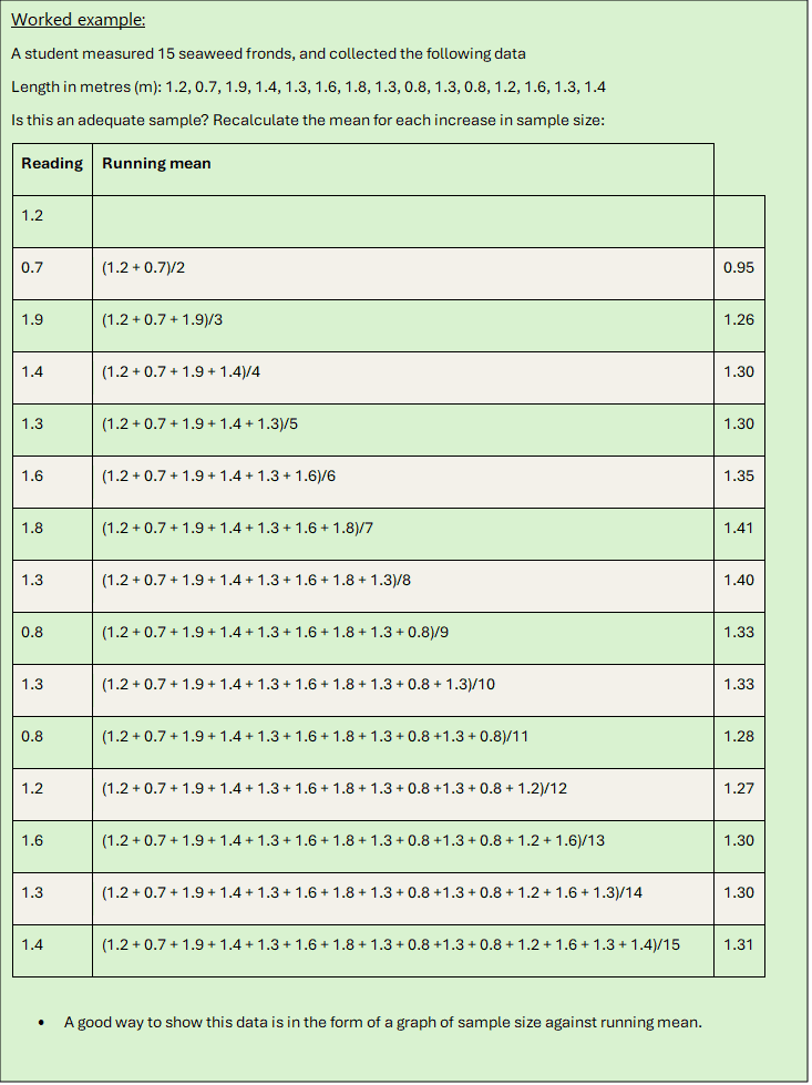
Running mean: justifying your sample size
It’s always a good thing to be able to say why you took a certain number of measurements. Why, for instance, did you count things in 30 rather than 20 quadrats?
The running mean is a simple technique that allows you to judge whether or not you have enough measurements or counts.
A more statistically valid approach to determine the number of repeats required is to calculate the running mean. By taking a number of repeat readings in a single location you can determine the number of samples required that will give you an average that takes in to account the natural variation that may occur at each sample point.
Begin by finding the mean of your first two readings, then the mean of the first three readings, then the mean of the first four readings and so on. The mean values will fluctuate each time, but will gradually settle within a closer limit, until the point is reached where adding to the sample only has a very small effect on the mean. You can assume at this point that the number of repeats is adequate.
Variables
The things that you are interested in measuring are called variables. There are two types:
- Independent variable is not affected by other things. It is independent of other variables.
- Dependent variable is affected by other things. It is dependent on other variables.
An independent variable causes a change in a dependent variable. A dependent variable cannot cause a change in an independent variable.
There are four measurement scales for variables:
- Nominal: variables that are not numerical,
e.g. categories like gender and ethnicity. - Ordinal: variables where order has meaning, but the difference between values is not important,
e.g. ranks like 1st, 2nd and 3rd, or the ACFOR scale. - Interval: variables where the difference between values is important,
e.g. actual numbers like the temperature in °C. - Ratio: Interval data with a natural (absolute) zero point.
Time in seconds has a ratio scale, but temperature in °C does not (since 0°C does not mean no heat).
Matched and unmatched data
Your data is matched if a piece of data from one set goes with only one piece of data from the other set. For example, you might be measuring temperature of the sea with depth. A specific temperature recording would only be associated with one specific depth.
Your data is unmatched if there is no reason to associate a piece of data from one set with any particular piece of data from the other set. For example, you might be measuring the heights of vegetation on trampled and untrampled parts of a path. There is no connection between any of the measurements from the trampled part and the untrampled part.
Statistical tests
There are four main statistical tests for biologists to know, these are…
- T-test
- Spearman’s rank correlation coefficient
- Chi-squared test
- Mann-Whitney U test
T-test
A T-test will tell you if the means of two sets of normally distributed, unmatched, continuous data, with interval level measurements are significantly different to one another.
For any T-test, the null hypothesis will be: There is no significant difference between the means of the two sets of data
See our video guide worked example here: Student T-test video:
Spearman’s rank correlation coefficient
Spearman’s rank correlation coefficient will tell you whether 2 variables are correlated. In other words, des one variable change as the other one changes?
It will tell you whether the relationship is positive (both go up together) or negative (one goes up as the other goes down) and the strength of any correlation. It assumes that any relationship is roughly a straight line one.
For any Spearman’s rank test, the null hypothesis will be: There is no significant correlation between the two variables.
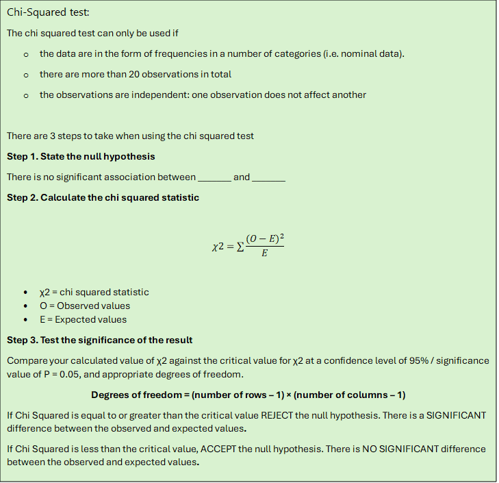
Chi-squared test
A chi-squared test can see if an observed set of data (which has to be counts of things in categories, or frequencies) differs significantly from what might be expected.
Chi squared is a statistical test that is used either to test whether there is a significant difference, goodness of fit or an association between observed and expected values.
For any chi-squared test, the null hypothesis will be: There is no significant difference between the observed and the expected frequencies.
Mann-Whitney U test
The Mann-Whitney U test tells you whether the median values of two sets of data are significantly different from one another.
It has the advantage that the data does not have to be normally distributed, and you can use it on small quantities of count data.
For any Mann-Whitney U test, the null hypothesis will be: There is no significant difference between the medians of the two sets of data.
