Method for High Energy Coasts

All Geography starts with someone going into the field to find out what’s there. This section will help you to gather the primary data (data you collect yourself) and secondary data (data collected by someone else) that will support your analysis and conclusions.

Type of data	Primary data collection technique	Secondary data collection source
Distribution of landforms in the landscape	Field sketching Photographs Mapping	Maps and aerial photographs Shoreline Management Plans
Shape of landforms (morphology)	Cliff surveys: profile, plan, degradation Shore platform surveys	Maps and aerial photographs Historical maps and photographs
Wave size, direction and frequency	Wave survey	Wave and wind data

Distribution of landforms in the landscape

1. Field sketching

The aim of field sketching is to produce a drawing which could be used by someone else as a guide to a landscape that they had never seen.

Find a comfortable and safe view point to sit down and draw. Record the grid reference and direction. A cardboard frame may be useful if the view is wide. Use a soft pencil (no harder than HB) and smooth paper. Once the preliminary sketch is complete, you may wish to use black ink and different grades of pencil to finish off the picture, but this requires more confidence.

A view is made up of “masses” (such as cliffs, buildings and trees). The first task is to draw the outline shape of each mass in the correct size, shape and position in relation to the other masses. To do this, it may help to divide the view up into the background (including the boundary line between land or sea and sky, middle ground or foreground. Start by drawing the background and work towards the foreground.

Many students draw slopes that are far too steep. Try holding a pencil or the edge of a book horizontally in front of you, then estimate the angle of elevation. As a rule of thumb, if you can walk up the slope without using your hands to steady yourself, then it is no steeper than around 22°. A slope marked as 25% (or 1 in 4) on roadsigns – about the maximum steepness that a car could easily drive up – has an angle of elevation of 14°.

It is also very easy to exaggerate the vertical scale. Measure true vertical or horizontal distances with the tip of the thumb on a pencil held out at arm’s length.

Shading is used to finish off the sketch. Emphasise valley sides and other slopes with faint lines that run up and down the slope. Steep cliffs can be shaded with near vertical lines. You can create the illusion of depth in the landscape by adding tone, best done by using a pattern of dots. The light parts of close objects are very light, and the shadowed parts are very dark. Distant objects are more uniform in tone.

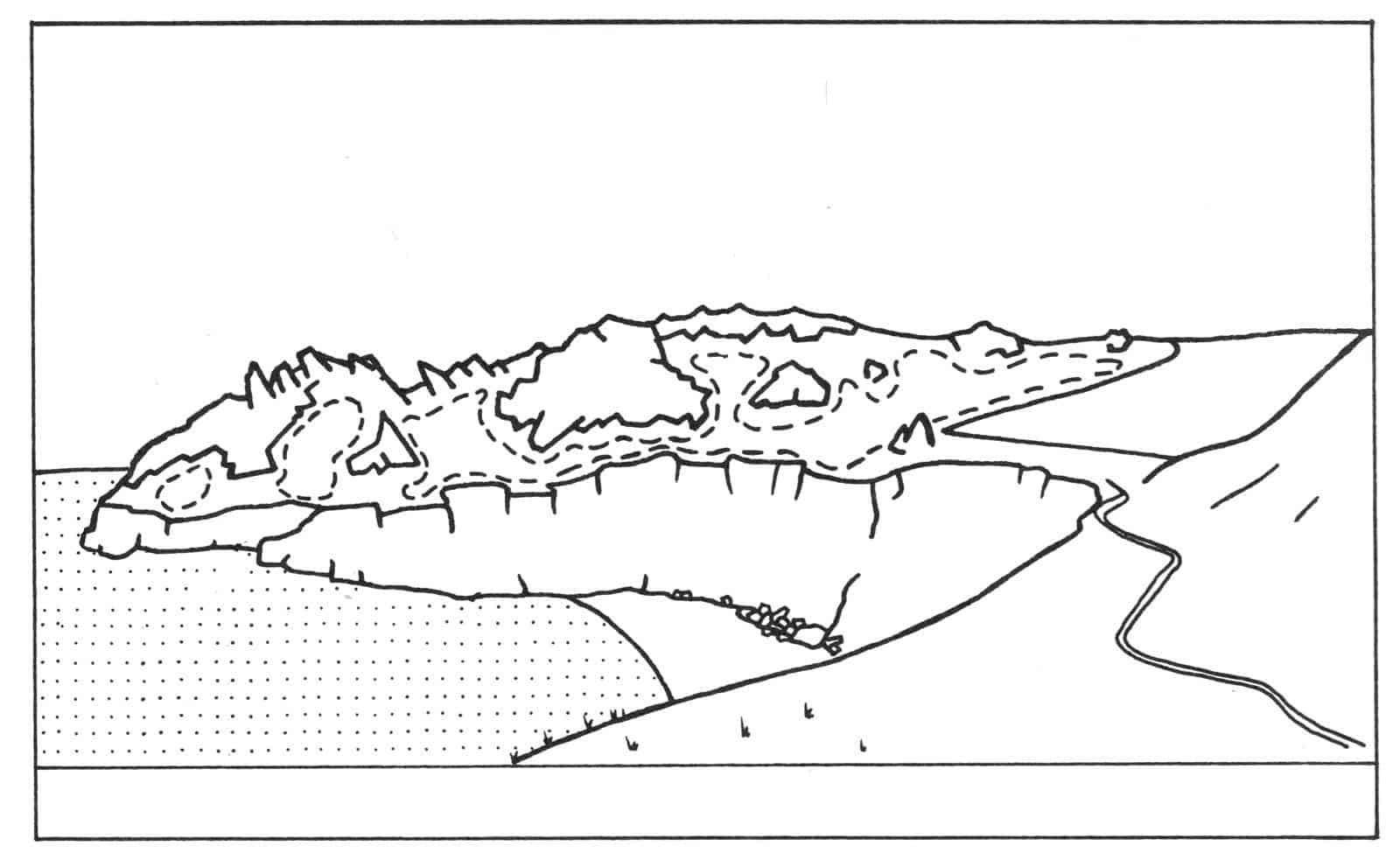
Annotate the view with descriptive and explanatory comments.The image above shows a field sketch of headlands, cliffs and shore platforms at Prawle Point in Devon. Shading and tone have been used.

2. Photographs

Don’t turn your project into a photo album. Instead use a small number of photographs that illustrate a particular feature of the landscape. Record the grid reference and direction for each photograph. It is a good idea to mark these on a base map. Annotate each photograph with descriptive and explanatory comments.

3. Mapping

Obtain a base map of the area. A 1:25 000 Ordnance Survey map is ideal. It is best to concentrate on a small length of coastline, such as a headland and bay sequence. Mark on the map the location and size of all landforms that you see.

Shape of landforms (morphology)

1. Cliff surveys: profile and plan

Broadly there are two aspects of a cliff to consider: the cliff profile (a vertical cross-section) and the cliff plan (the shape of the cliff when viewed from the air).

Although you may be able to measure the height and depth of a wave-cut notch (if present), do not attempt to climb cliffs directly

Data on the cliff profile can be made by carrying out field measurements at the base of the cliff. Divide the cliff face into 1-4 segments, each separated by a break of slope.

Use a clinometer to find the angle of elevation from the ground to the point of each break of slope.

To find the height each cliff segment, use a large scale map to find the total height of each cliff. Estimate the percentage of the total cliff height that makes up each cliff segment. For example, if a cliff is 20m in height and a single cliff segment is approximately one half of the height of the whole cliff, then the height of the cliff segment is approximately 10m.

The field data can be used to plot slope profiles for the cliffs. Make a justified decision on how many slope profiles that you take.

Data on the cliff plan can be collected from aerial photographs.

2. Cliff degradation

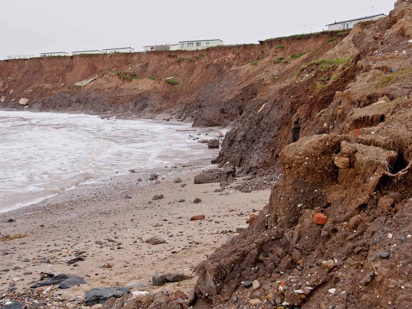
Construct and an index of cliff degradation. Look for material at the base of the cliffs (such as rock fall material or slumped mud) plus any signs of mass movement or sub-aerial weathering further up the cliff (such as cracks). Fresh rock and mud surfaces without vegetation can indicate recent activity.

Example of a index of cliff degradation for a length of boulder clay cliffs

Score 0 = stable cliffs with 75% vegetation cover

Score 5 = cliff toe covered in slumped mud with 0% vegetation cover

3. Shore platform surveys

There is a risk of being trapped by the rising tide when working on shore platforms. Make sure that there is at least one clear escape route. Check tide tables and only carry out fieldwork on a falling tide, ideally starting no later than three hours before low tide level.

(a) Slope angles

Data on the width and gradient of shore platforms can be collected by measuring slope angle over a series of transects running from the seashore to the base of cliffs. Use a clinometer, ranging poles and tape measures to record slope angle.

On a shore platform, height above low tide may be more important than horizontal distance. Use tide tables to identify the time of low tide, then use this as a reference point. You can also use the tide tables to work out how much higher your reference point is from extreme low water spring tide (ELWS) level.

Height levelling with an optical level needs two people. The first person stands at the water’s edge with an optical level placed so that the eye piece is level with the top of a metre rule. This first person asks a second person to move up the rocky shore until the point that the bottom of the second person’s feet become visible through the eye piece. The rise from the two people is therefore 1 metre. Repeat the procedure to continue measuring the height.

(b) Surface features: potholes, pools and runnels

Recording surface features is useful if you are making a detailed survey of a single shore platform. Devise a sampling strategy – either random, systematic or stratified – to sample different parts of the shore platform. At each site place a 1 metre square quadrat on the ground. Here are some suggestions of features that you could measure within each quadrat:

(i) Vertical dissection: how smooth is the ground surface? Use a metre rule to measure the difference between maximum height and minimum height at regular intervals. Mean, range and standard deviation can be calculated from the results for each site, or you could compare different areas of the shore platform.

The roughness ratio compares the straight line distance between the edge of the quadrat with the actual ground distance following all the indentations. If you have measured the difference between maximum and minimum height, it is possible to calculate the actual ground distance using trigonometry.

Or you could lay a tape closely onto the rock from one point to another following all the indentations. Carefully measure out 1 metre, and mark the start and end points. Now stretch the tape tightly between these start and end points. Measure the straight line distance. The roughness ratio is calculated as

\(\mathsf{roughness\;ratio = \frac{distance\;following\;all\; indentations}{distance\;with\;tape\;stretched\;tightly}}\)

For a smooth surface the roughness ratio will equal 1. The rougher the surface, the closer the ratio will be to zero.

(ii) Density of pools and pits: how many surface depressions are there? Count the number of pools and pits in each metre square. Calculate the density as:

\(\mathsf{density\;of\;pools\;and\;pits = \frac{number\;of\;pools\;and\;pits}{area\;sampled}}\)

(iii) Area of pools and pits. A gridded quadrat is the easiest way to collect this information in the field. Or you could measure the dimensions of each pool and pit. You could then calculate the mean area of the pools and pits. Or you calculate the percentage of the area of the quadrat that is made up of pools and pits.

(iv) Surface texture: how smooth is the ground surface? This can be assessed by touch. Rub a single finger over the rock surface. Use the notation 0, +, ++ and +++ to classify the surface on a scale from completely smooth (you cannot detect individual grains) to coarse (you can feel grains wider than 1-2mm). You could also use the 0, +, ++ and +++ scale to classify the hardness of the surface on a scale from hard (e.g. surface cannot be scratched with a screwdriver) to loose (e.g. surface crumbles when rubbed with a finger).

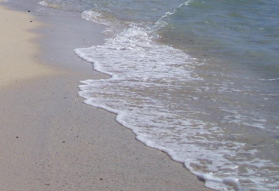
Wave surveys

Wave action is one of the key factors shaping coastal landforms. High energy waves have a high frequency and height, and tend to be destructive (contribute to erosion). Low energy waves have a low frequency and height and tend to be constructive (contribute to accretion). However, the pattern of waves over time is a more reliable predictor of the processes of erosion and accretion than the characteristics of individual waves.

1. Wave height and frequency

Wave height is determined by three variables: wind speed, wind duration (how long the wind blows), and fetch (the distance over water that the wind blows in a single direction).

Wave height can be estimated by using a groyne or other marker on the beach to judge the height of at least 20 waves. Calculate mean wave height.

Wave frequency is defined as the number of waves passing a fixed point in a specified amount of time. It can be estimated by counting the number of waves breaking on the shore in 10 minutes. Calculate mean wave frequency per minute.

2. Comparing the swash and the backwash

Swash describes the water that flows towards the beach after a wave breaks. Backwash describes the water than runs back down the beach. A high energy wave tends to have a weak swash and a strong backwash, whereas a low energy wave tends to have a strong swash and a weak backwash.

Monitor the waves breaking on the shore for 10 minutes. Measure the time (in seconds) that the swash of each wave moves upwards. Note whether the backwash of each wave either drains into the beach material, runs back down the shore before the next wave arrives or interferes with the swash of the next wave. What might these observations tell you about the relative strength of the swash and the backwash?

Secondary data sources

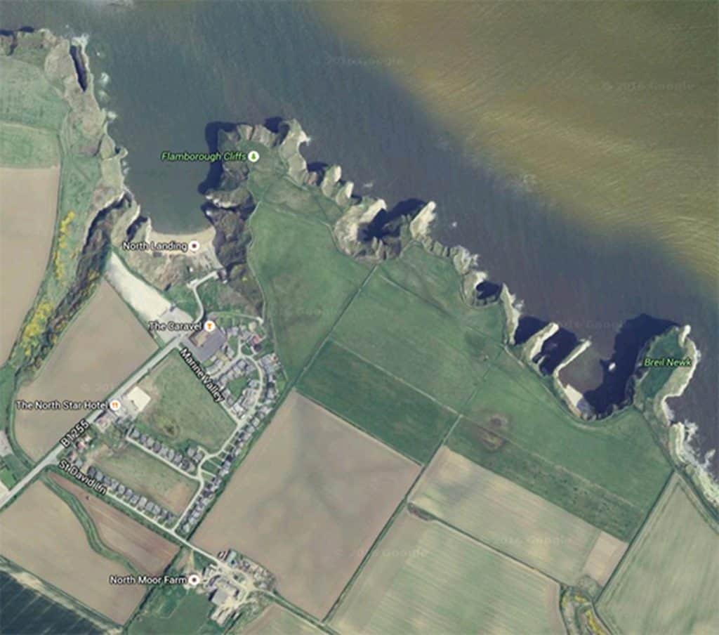
1. Maps and aerial photographs

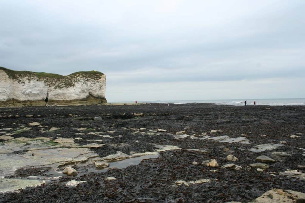
Maps and aerial photographs (including Google Earth) are useful for assessing the planform of coastal landforms, such as cliffs. For example, using the measurement tools on ArcGIS or Bikemap, the length, width, shape and area of Flamborough Head in East Yorkshire can be judged.

2. Historic maps and photographs

Old Ordnance Survey maps from across England, Wales and Scotland can be browsed at the National Library of Scotland archive

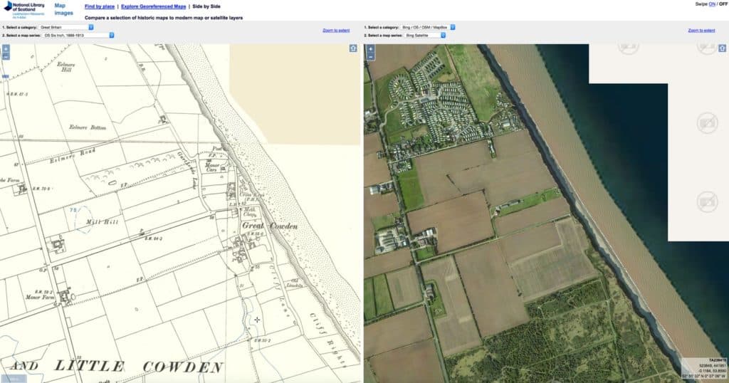
Use the option “Side by Side” to compare historic maps with present-day maps and aerial photographs. Below shows an example of how the large scale maps showing field boundaries could be used as a source of data on how much land has been eroded around the East Yorkshire village of Great Cowden since the early 20th century. Much of the village shown in the 1908 map (on the left) is no longer in existence in the present-day aerial photo (on the right).

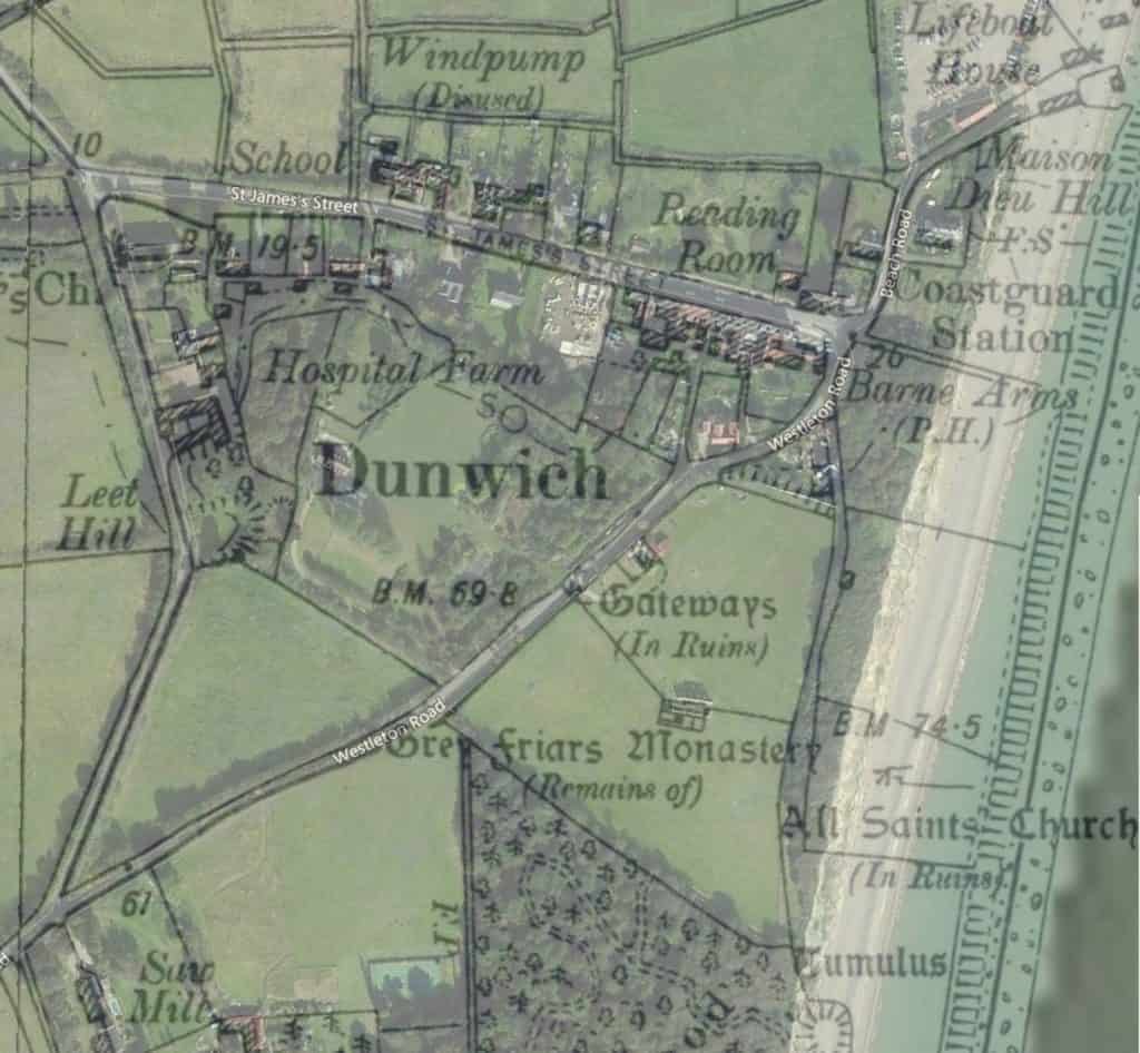
Historic maps can also be overlaid over present-day views. The example below shows a 1905 map overlaid over a recent aerial view. The loss of land, roads and buildings on the eastern side of the view is clear. Historic erosion rates could be measured from these views.

3. Wave and wind data

This can be found at

• Magic Seaweed
• National Data Buoy Centre
• Channel Coastal Observatory

4. Shoreline management plans

Shoreline management plans are an essential source to find our more about about erosion and other coastal processes in your chosen length of coastline.

Projections of coastal flooding as a result of sea level rise can be modelled using Flooding Firetree.

---