All Geography starts with someone going into the field to find out what’s there. This section will help you to gather the primary data (data you collect yourself) and secondary data (data collected by someone else) that will support your analysis and conclusions.
| Type of data | Primary data collection technique | Secondary data collection source |
|---|---|---|
| Distribution of landforms in the landscape | Field sketching Photographs | Maps and aerial photographs BRITICE Geological maps |
| Shape of landforms (morphology) | Cross-sections Mapping | Maps and aerial photographs BRITICE Geological maps |
| Ice and meltwater movement | Sediment analysis: size, shape, sorting Mapping ice direction | BRITICE Geological maps |
| Periglacial processes | Field sketching Photographs Sediment analysis: size, shape, sorting | BRITICE Geological maps |
| Scree | Field sketching Photographs Sediment analysis: size, shape, sorting | BRITICE Geological maps |
Distribution of landforms in the landscape
1. Field sketching
The aim of field sketching is to produce a drawing which could be used by someone else as a guide to a landscape that they had never seen.
Find a comfortable and safe view point to sit down and draw. Record the grid reference and direction. A cardboard frame may be useful if the view is wide. Use a soft pencil (no harder than HB) and smooth paper. Once the preliminary sketch is complete, you may wish to use black ink and different grades of pencil to finish off the picture, but this requires more confidence.
A view is made up of “masses” (such as hills, cliffs, buildings and trees). The first task is to draw the outline shape of each mass in the correct size, shape and position in relation to the other masses. To do this, it may help to divide the view up into the background (including the boundary line between land and sky, middle ground or foreground. Start by drawing the background and work towards the foreground.
Many students draw slopes that are far too steep. Try holding a pencil or the edge of a book horizontally in front of you, then estimate the angle of elevation. As a rule of thumb, if you can walk up the slope without using your hands to steady yourself, then it is no steeper than around 22°. A slope marked as 25% (or 1 in 4) on roadsigns – about the maximum steepness that a car could easily drive up – has an angle of elevation of 14°.
It is also very easy to exaggerate the vertical scale. Measure true vertical or horizontal distances with the tip of the thumb on a pencil held out at arm’s length.
Shading is used to finish off the sketch. Emphasise valley sides and other slopes with faint lines that run up and down the slope. You can create the illusion of depth in the landscape by adding tone, best done by using a pattern of dots. The light parts of close objects are very light, and the shadowed parts are very dark. Distant objects are more uniform in tone.
Annotate the view with descriptive and explanatory comments.
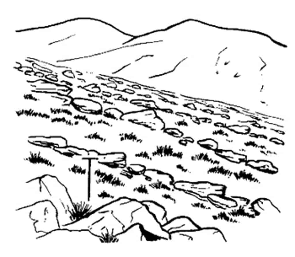
Example of using sketching to illustrate a particular upland landform: periglacial stone stripes in the Rhinog mountains, Snowdonia. Notice how most detail has deliberately been left out, especially in the background.
2. Photographs
Don’t turn your project into a photo album. Instead use a small number of photographs that illustrate a particular feature of the landscape. Record the grid reference and direction for each photograph. It is a good idea to mark these on a base map. Annotate each photograph with descriptive and explanatory comments.
Shape of landforms (morphology)
3. Cross sections
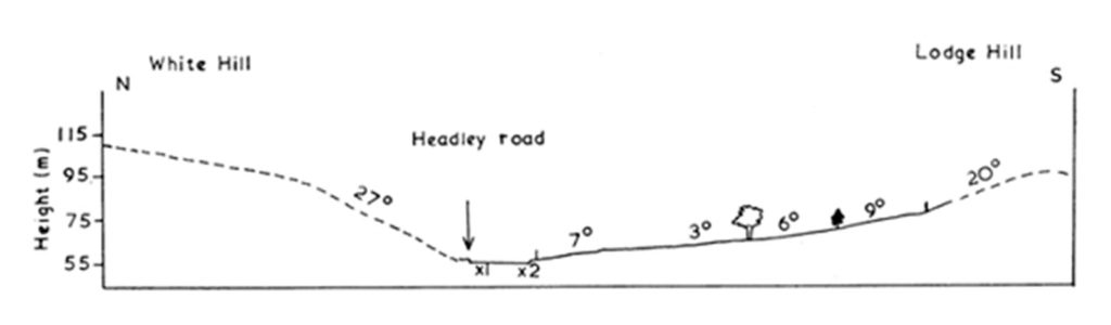
Cross sections use distance and angle measurements to help you investigate the shape of the landforms. You may wish to take a cross-section of a U-shaped valley or a corrie, for example.
Follow a straight transect line. Split the line into segments where the slope angle changes. Each reading is taken from from break of slope to break of slope.
- Person A holds a ranging pole
- Person B stands holding a second ranging pole further uphill where there is a break of slope
- The distance between the two ranging poles is measured using a tape measure
- The angle between matching markers on each ranging pole is measured using a clinometer
- Repeat this process at each break of slope until the edge of landform is reached
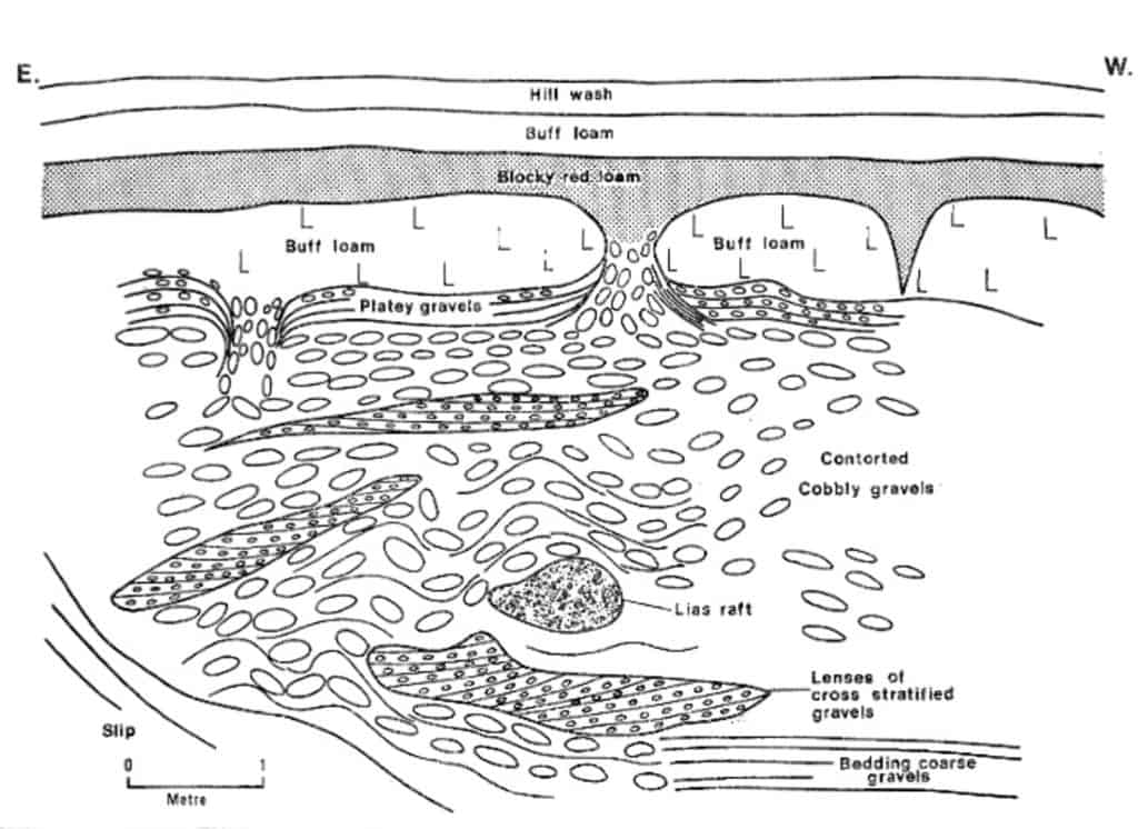
You can also sketch exposures of sediment. The sketch below shows a cross-section through fluvioglacial deposits in west Somerset, exposed by coastal erosion of cliffs.
4. Mapping
Obtain a base map of the area. A 1:25 000 Ordnance Survey map is ideal. It is best to concentrate on a small area, of no more than a few square kilometres. Try to walk over the whole area. Mark on the map the location and size of all landforms that you see. These might include glacial erratics, mounds of moraine, drumlins and eskers.
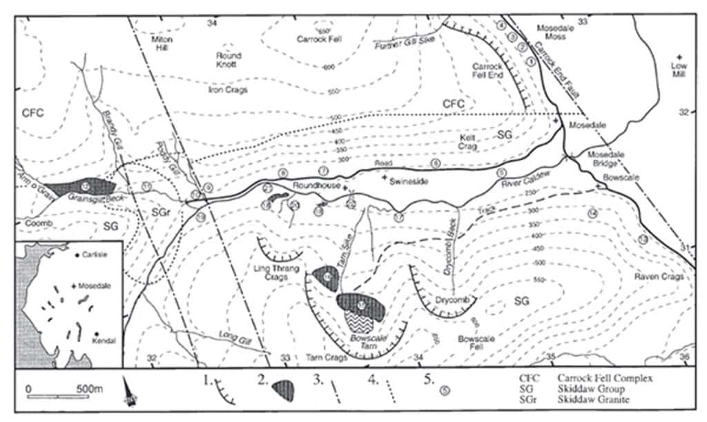
In this example, a base map of part of Mosedale in the Lake District has been annotated with numbers 1-20. Each of these features is described and explained in the key.
Ice and meltwater movement
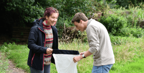
5. Sediment analysis: size
Use a trowel or soil augur to take sediment samples from below the soil. Each sample should be placed in a sealed plastic bag and accurately labelled.
Use rules or calipers to measure the a, b and c axes of each pebble.
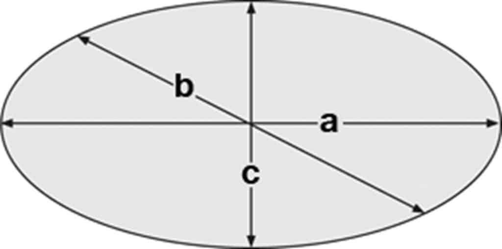
The a-axis is the longest axis
The b-axis is the widest axis at right angles to the a-axis.
The c-axis is the shortest axis.
6. Sediment analysis: shape
The simplest way to record pebble shape is to classify the stone as very angular, angular, sub-angular, sub-rounded, rounded or very rounded using a Power’s Scale of Roundness. This is judged by eye.

Using a protractor or concentric circle card, measure the minimum radius of curvature. This is the sharpest corner on the a-axis.
Alternatively use the pebble size measurements (a, b and c axes) to calculate Zingg’s shape classification, Krumbein’s Index of Sphericity or Cailleux’s Flatness Index (see Data Analysis). Use the a-axis and minimum radius of curavture to calculate Cailleux’s Roundness Index.
7. Sediment analysis: sorting
Use a set of graduated sieves can be used to sort sediment samples into different size categories (in millimetres or as phi sizes).
The sieves are arranged in decreasing mesh diameter with the largest at the top. The sediment sample is placed in the top sieve then the sieves are shaken to sort the sediment into the various sieves. The mass of sediment in each sieve is measured using scales and the percentage of the total sample can be calculated.
8. Mapping ice direction
It is fairly easy to tell the direction of ice flow for a present-day glacier, but not so easy to trace the direction in a deglaciated landscape in Britain. Instead you have to look for what evidence has survived. There are four main sources of evidence you could consider. These are a combination of glacial erosion and glacial deposition.
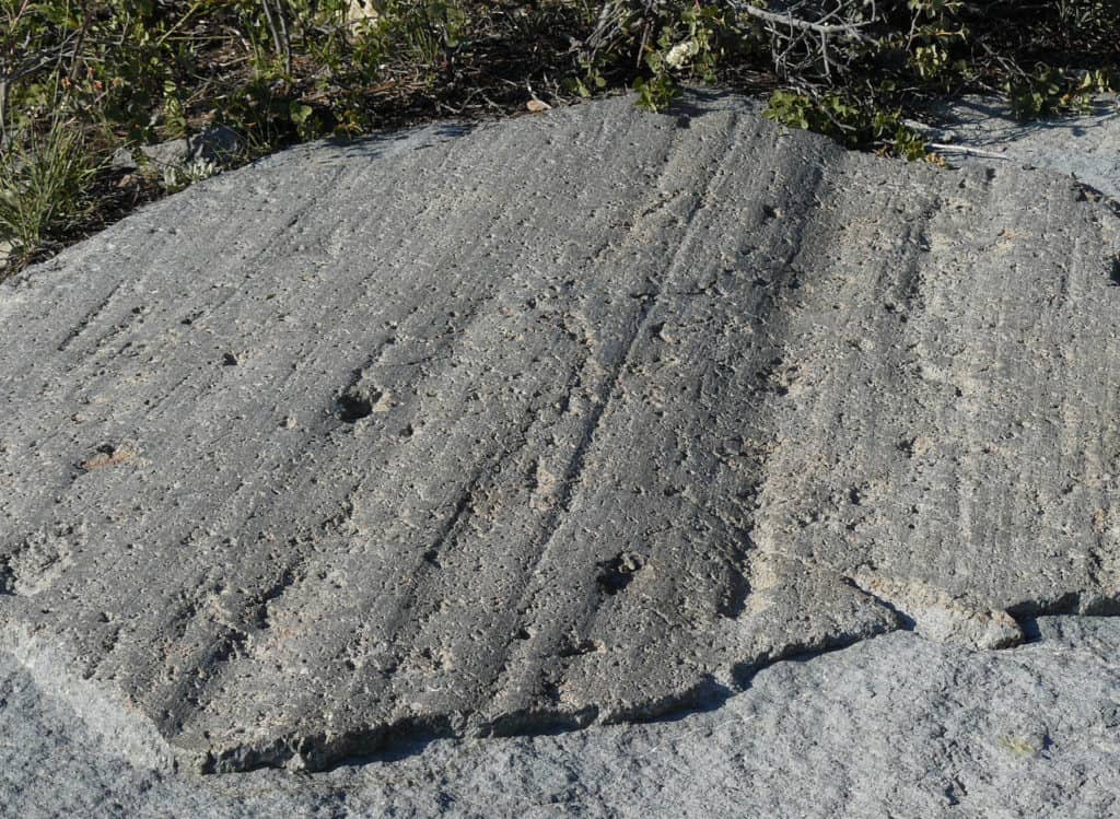
(a) Striations: scratches on glacially eroded bedrock surfaces, produced by rock embedded in the ice as it moves across. Using a compass or protractor, note the orientation of the striations. Striations are not always easy to identify, and it is possible to confuse them with joints and faults in the rock.
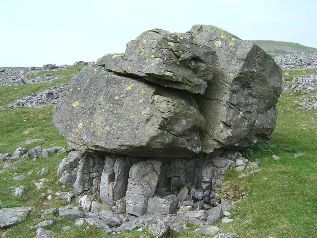
(b) Rock provenance: working out where the rocks deposited by the glacier have come from. Glacial erratics (blocks of rock which are different in rock type to the country rocks of the area) are a good place to start. Map the location of large boulders. Use secondary sources to work out from where they might have originated.
(c) Orientation of small-scale landforms: including drumlins and roche moutonnees. A drumlin is a landform of glacial deposition. The high and steeply-sloping stoss side is the upstream side, while the gently sleeping lee side is the downstream side. A roche moutonnee is a landform of glacial erosion. Here the gently-sloping stoss side is the upstream side, while the steeply-sloping stoss side is the downstream side.
(d) Stone orientation: find the orientation of fragments in glacial deposits. It is easiest to do this for a recently exposed till face, such as besides a new farm track or a meandering stream. Without disturbing the till face, sample at least 50 protruding pebbles. Use a compass to find the direction that each pebble points. The long axis of the pebble should be parallel to the direction of ice flow.
Secondary sources
1. BRITICE
BRITICE is a map and GIS database of glacial landforms in England, Wales and Scotland. This includes moraines, eskers, drumlins, ice-dammed lakes and meltwater channels. You can download Google Earth map layers.
2. Geological maps
Glacial, fluvioglacial and periglacial deposits have been mapped at the Geology of Britain viewer. Zoom to a location, then select “Superficial only” for the surface geology.
The British Geological Survey has produced two online resources for exploring the lowland glaciation of two sites: Anglesey and the Blakeney Esker in Norfolk
Secondary and Further Education Courses
Set your students up for success with our secondary school trips and courses. Offering excellent first hand experiences for your students, all linked to the curriculum.
Group Leader and Teacher Training
Centre-based and digital courses for teachers